Monitor the consumption of M3 node during an experiment
![]() Difficulty: Medium
Difficulty: Medium
![]() Duration: 20 minutes
Duration: 20 minutes
Prerequisites: Configure SSH Access / Submit an experiment with M3 nodes using the web portal
Description: Each node of an experiment is managed by its Control Node (users have no access to it), that interacts passively or actively. It monitors node consumption, power radio signal (RSSI) and selects power supply (battery or DC through POE). A Profile represents the Control Node configuration during the experiment. The aim of this tutorial is to create a profile for monitoring consumption and launch an experiment with a firmware that turns on/off red, blue and green LEDs (1Hz period)
- Log into the Webportal
- Select the Resources / Monitoring profiles tab
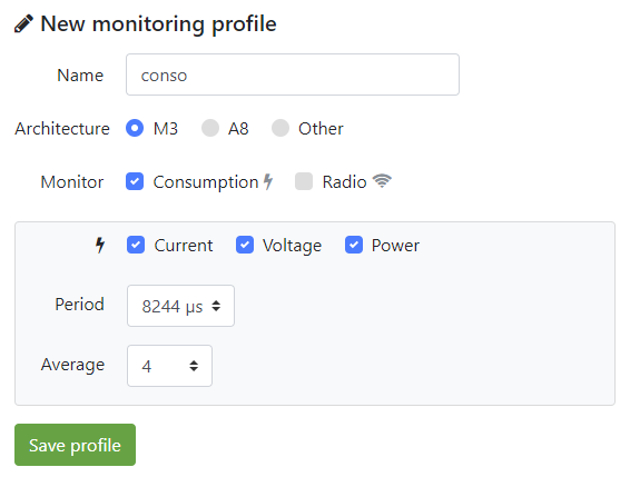
- Click the New profile button to create a new profile
- Set a profile Name, the M3 Node architecture, and all the Consumption checkboxes (current, voltage, power) with:
- Period = 8244 µs
- Average = 4
- Save this profile.
- This setting will give you a sampling period of P = 8.244 ms * 4 * 2 = 65.95 ms (see below for more informations about the sampling period).
- Submit a new experiment
- Duration : 10 minutes and select “As soon as possible”
- Choose one node:
- Select nodes “by node properties”
- Select Archi = M3 (at86rf231) / Site = Grenoble / Quantity = 1 / Mobile = no
- Click “Add to experiment”
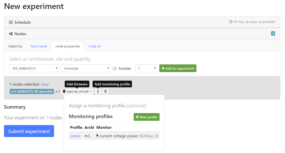
- Firmware association: use this tutorial binary firmware file. (click button Add Firmware (microship icon next to the node))
- Monitoring profile association: use the profile you have created earlier. (click button Add monitoring (thermometer icon))
- Click on the experiment in the list, and make a note of the node id, while you wait for the experiment to become running.
- Connect to the SSH fronted of Grenoble with X11Forwarding
ssh -X <login>@grenoble.iot-lab.info
- The consumption measure values are stored in your home folder in .oml files. As we use caching mechanism, you must wait that you have content in the file.
<login>@grenoble:~$ less ~/.iot-lab/<experiment id>/consumption/m3-<id>.oml
protocol: 4
domain: 1621
start-time: 1379945917
sender-id: m3-3
app-name: control_node_measures
schema: 0 _experiment_metadata subject:string key:string value:string
schema: 1 control_node_measures_consumption timestamp_s:uint64 timestamp_us:uint32 power:double voltage:double current:double
content: text

1.341009        1       1       1379945918      303436  0.053461        3.272500        0.016347
1.341392        1       2       1379945918      307892  0.053232        3.273750        0.016270
1.341448        1       3       1379945918      312317  0.053384        3.272500        0.016322
See the profile measure table below for more informations.
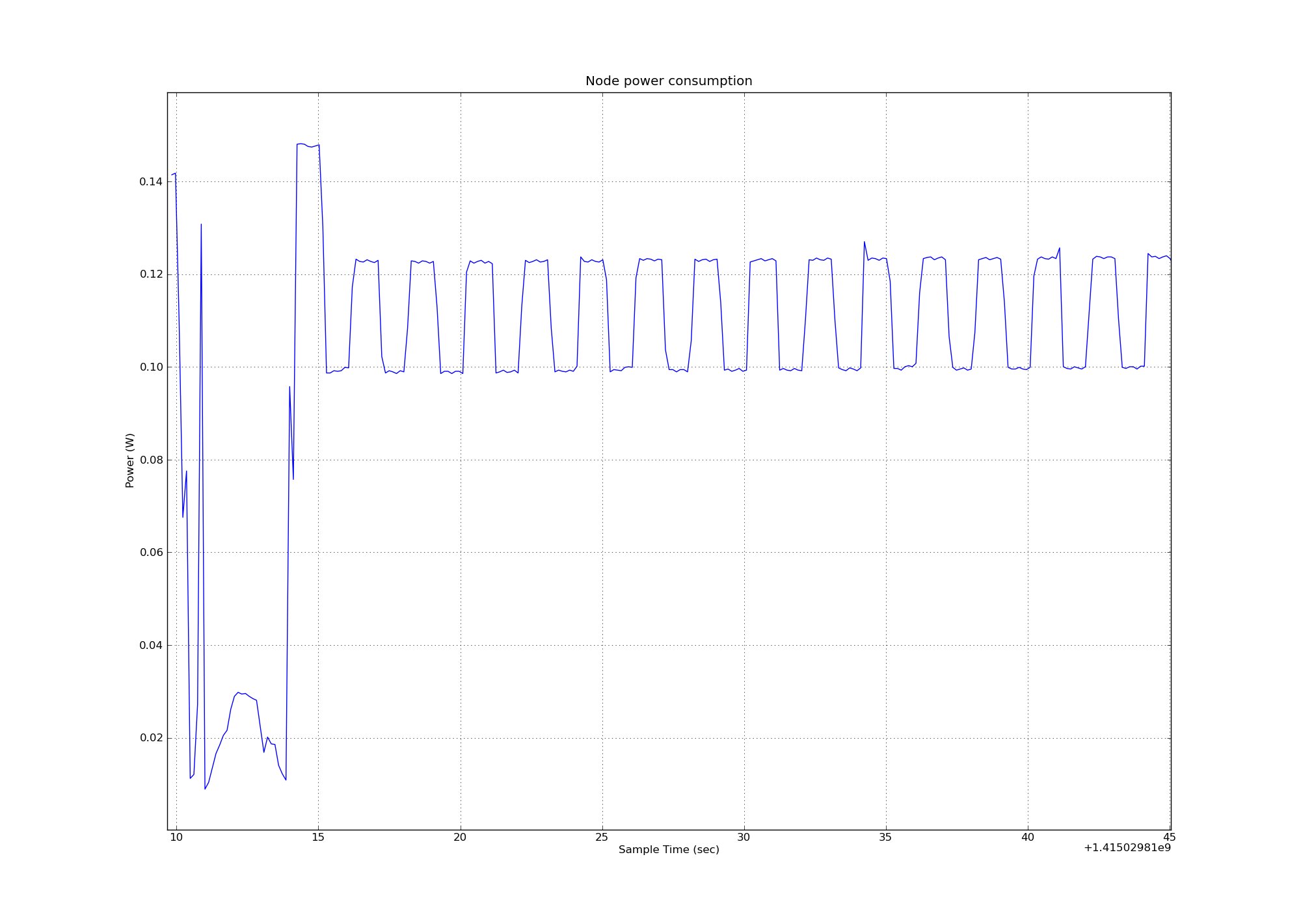
- Plot your file using the oml_plot.py script file
<login>@grenoble:~$ plot_oml_consum -p -i ~/.iot-lab/<experiment id>/consumption/m3-<id>.oml
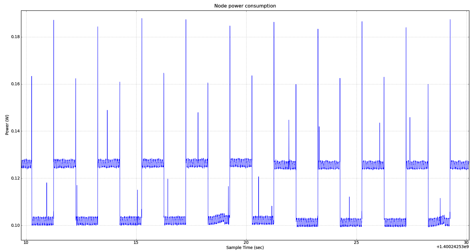
You may observe oscillations corresponding to the 1Hz LED(s) blinking. It is also possible to measure the current on each LED which is theoretically equal to 2.4 mA.
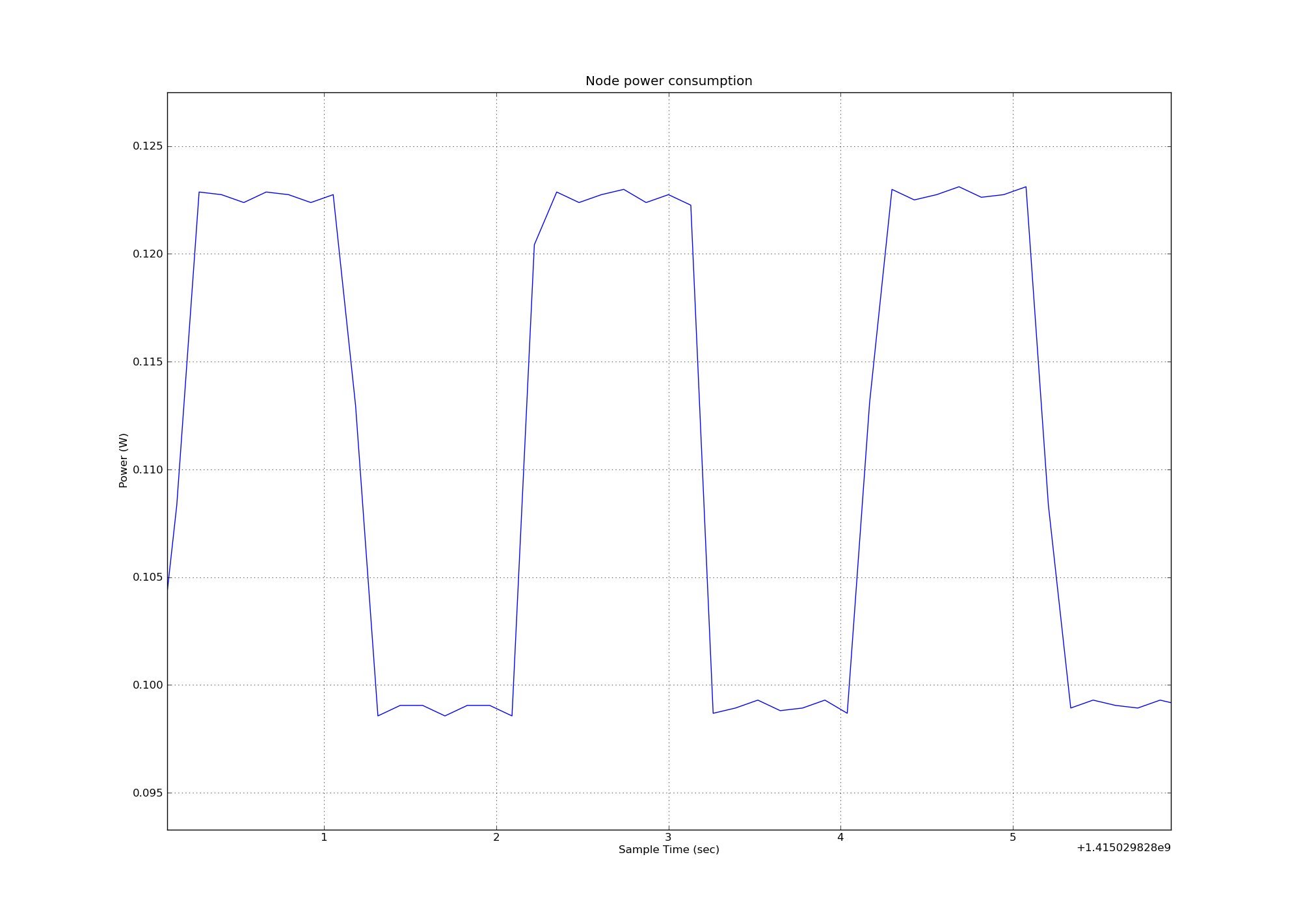
- Repeat the operations 3. to 7. to measure the LED consumption, changing the monitoring sample period parameters given in 4. By choosing a smaller sample period (Period = 1100 µs = 1.100 ms ; Average = 1 ; Sample Period = 1.100 * 1 * 2 = 2.200 ms), you will observe that the signal measure noise is not filtered (see figure below).
Additional details
Averaging and Conversion Time Considerations
The M3 node is connected on a gateway which measures its consumption through resistor shunts and an INA226 current/power monitor component.
The INA226 has programmable conversion times for both the shunt voltage and bus voltage measurements. The conversion times (CT) for these measurements can be selected from as fast as 140μs to as long as 8.244ms. The conversion time settings, along with the programmable averaging mode (AV), allow the INA226 to be configured to optimize the available timing requirements in a given application. The periodic measure (PM) is then given by the formula:
PM = CT * AV * 2.
There are trade-offs associated with the settings for conversion time and the averaging mode used. The averaging feature can significantly improve the measurement accuracy by effectively filtering the signal. A greater number of averages enables the INA226 to be more effective in reducing the noise component of the measurement.
For example, if a system requires that data be read every 4ms, the INA226 could be configured for a non filtered signal with the conversion times set to 2116 μs and the averaging mode set to 1. This configuration results in the data updating approximately every
4.23 ms = 2.116 * 1 * 2.
With a configuration for a filtered signal, the conversion times can be set to 204 μs and the averaging mode can be set to 10 in order to have a periodic measure of
4.08 ms = 204 * 10 * 2
Profile measure table
| M3 node | Measure | Unit |
|---|---|---|
| Consumption | current voltage power |
ampere volt watt |
| Radio | RSSI | dBm |