Consumption monitoring
Consumption monitoring is an optional feature which measures the energy usage of your experiment nodes. It refers to the Control Node dedicated hardware installed on the IoT-LAB node to enable the monitoring. It provides you an efficient passive monitoring solution which helps you to design IoT protocols or applications with low-power devices. In this documentation you will learn how to create a Profile monitoring configuration and enable it for your experiment. Moreover you will figure out how to get and analyse the monitoring data.
Create a monitoring profile
You have two ways to create a monitoring Profile, the IoT-LAB Webportal or CLI command-line tools. In both cases you must create a Profile with a name, M3 architecture and the following configuration:
- Monitor consumption: current, voltage and power.
- Period: 8244 µs
- Average: 4
These settings will give you a sampling period of P = 8.244 ms * 4 * 2 = 65.95 ms. View this section for additional informations.
In the Webportal go to the Resources Monitoring page and click New profile button.
With command-line tools use these commands:
$ iotlab-auth -u <login> # optionally store your credentials if you haven't done it before.
$ iotlab-profile addm3 -n <profile_name> -voltage -current -power -period 8244 -avg 4
Launch an experiment
To illustrate the consumption monitoring we will launch an experiment with:
- a duration of 5 minutes
- one M3 node on Grenoble site
- a firmware flashing LED(s) with a frequency of 1Hz
- the consumption monitoring profile we have just created.
In the Webortal go to the New Experiment page and select nodes by node properties (one M3 node on Grenoble site) and attach the preset firmware (iotlab_m3_tutorial) and the consumption monitoring profile.
You can note that it’s possible to have a different monitoring configuration for each node of your experiment.
With command-line tools use these commands:
$ wget https://iot-lab.github.io/assets/firmwares/tutorial_m3.elf .
$ iotlab-experiment submit -d 5 -l 1,archi=m3:at86rf231+site=grenoble,tutorial_m3.elf,<profile_name>
$ iotlab-experiment wait
$ iotlab-experiment get -ni
Analyse monitoring data
The monitoring data is stored on the frontend server in your home directory. You can find it in the ~/.iot-lab/<exp_id>/consumption/ directory. We use the OML measurement library and you can find a file m3_<id>.oml for each monitored nodes.
Don’t worry if you have empty files, OML library performs caching. You have to wait a little while or manually stop the experiment to flush the cache.
Go to the frontend and view the monitoring OML file content:
$ ssh -X <login>@grenoble.iot-lab.info # -X option enables X11 forwarding
<login>@grenoble:~$ less ~/.iot-lab/last/consumption/m3_<id>.oml # .iot-lab/last is a symlink to your last experiment directory .iot-lab/<exp_id>
protocol: 4
domain: 1621
start-time: 1379945917
sender-id: m3-3
app-name: control_node_measures
schema: 0 _experiment_metadata subject:string key:string value:string
schema: 1 control_node_measures_consumption timestamp_s:uint64 timestamp_us:uint32 power:double voltage:double current:double
content: text

1.341009        1       1       1379945918      303436  0.053461        3.272500        0.016347
1.341392        1       2       1379945918      307892  0.053232        3.273750        0.016270
1.341448        1       3       1379945918      312317  0.053384        3.272500        0.016322
We provide an OML plotting tool which helps you to analyse monitoring data.
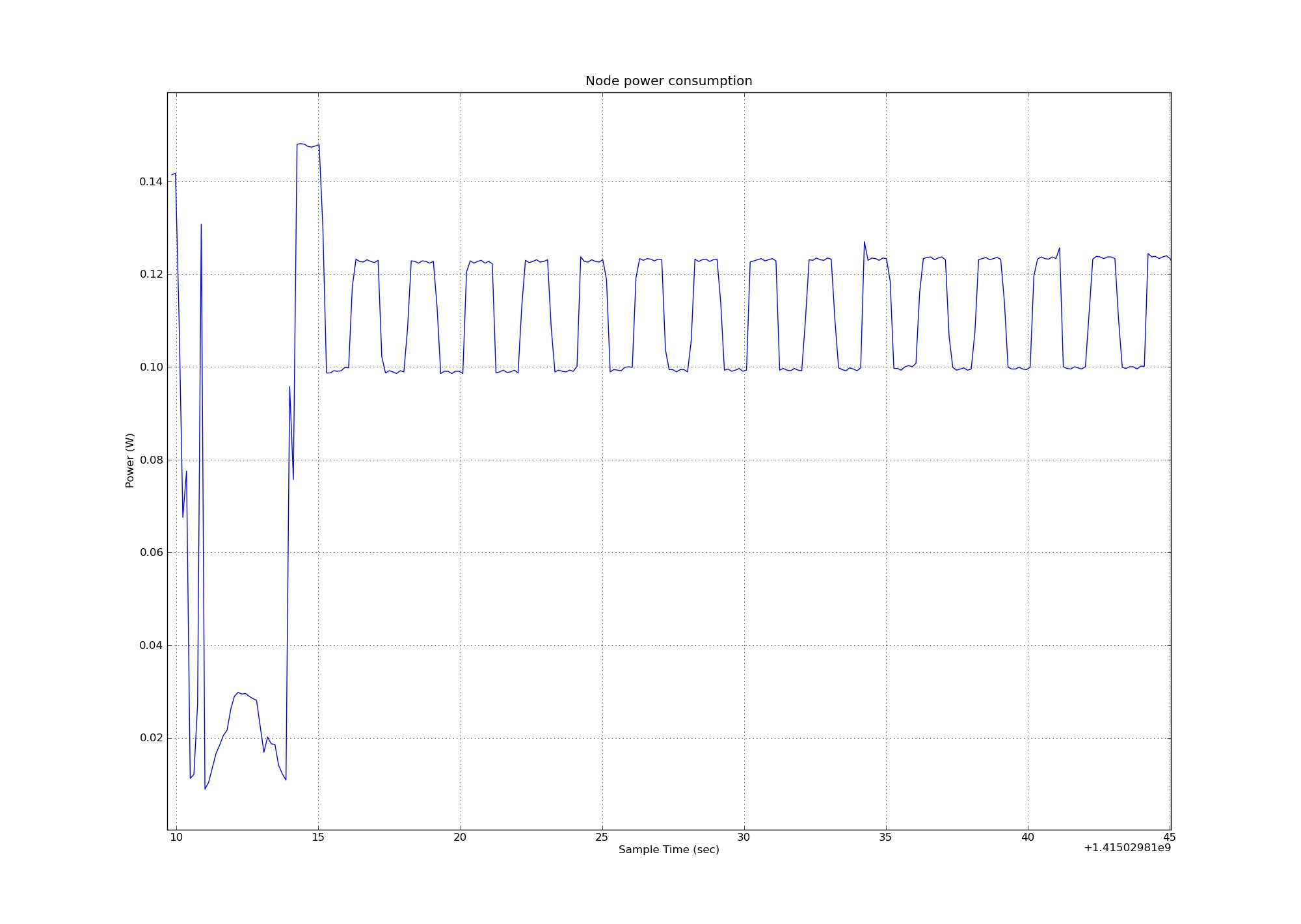
<login>@grenoble:~$ plot_oml_consum -p -i ~/.iot-lab/last/consumption/m3_<id>.oml
You may observe oscillations corresponding to the 1Hz LED(s) flashing. It is also possible to measure the current on each LED which is theoretically equal to 2.4 mA.
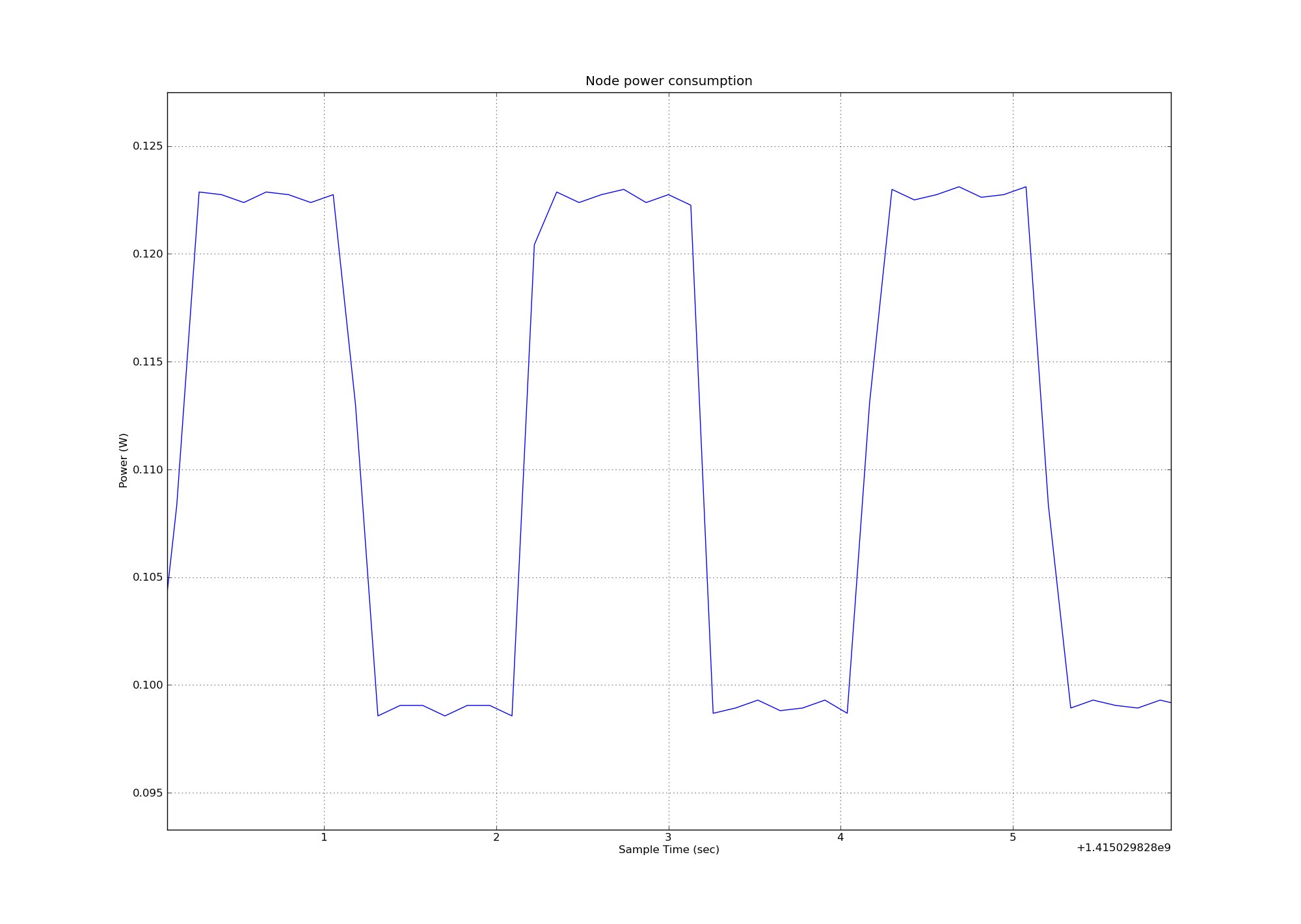
A zoom of the previous plot to see the one second period.
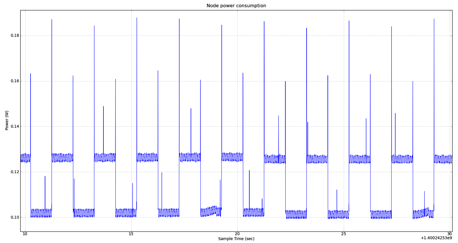
We join you an example of plot with a smaller sample period (2.200 ms = Period 1100 µs * Average 1 * 2). You can observe that the signal measure noise is not filtered.
Additional informations
The consumption of your node is measured through an INA226 hardware component . The INA226 has programmable conversion times for two measurements, the shunt voltage and the power supply bus voltage. The conversion times (CT) for these measurements can be selected from as fast as 140μs to as long as 8.244ms. The conversion time settings, along with the programmable averaging mode (AV), allow the INA226 to be configured to optimize the available timing requirements in a given application. The periodic measure (PM) is then given by the formula:
PM = CT * AV * 2
There are trade-offs associated with the settings for conversion time and the averaging mode used. The averaging feature can significantly improve the measurement accuracy by effectively filtering the signal. A greater number of averages enables the INA226 to be more effective in reducing the noise component of the measurement.
For example, if a system requires that data be read every 4ms, the INA226 could be configured for a non filtered signal with the conversion times set to 2116 μs and the averaging mode set to 1. This configuration results in the data updating approximately every 4.23 ms = 2.116*1*2
With a configuration for a filtered signal, the conversion times can be set to 204 μs and the averaging mode can be set to 10 in order to have a periodic measure of
4.08 ms = 204*10*2
| Measure | Unit |
|---|---|
| current | ampere |
| voltage | volt |
| power | watt |